Gå til hovedindhold

Hvordan skjules kun en del af celleværdien i Excel?

doc skjul delvist 1
Antag at du har et ark med nogle generelle oplysninger om personalet, men nogle er private, såsom personnumre. Nu vil du skjule en del af disse socialsikringsnumre som vist nedenfor, hvordan kan du hurtigt løse det?

Skjul socialnumre delvist med Format Cells

Delvist skjul tekst eller tal med formler

pil blå højre boble Skjul socialnumre delvist med Format Cells

For at skjule en del af personnumre i Excel kan du anvende Format celler for at løse det.

1. Vælg de numre, du vil skjule delvist, og højreklik for at vælge formater celler fra genvejsmenuen. Se skærmbillede:
doc skjul delvist 2

2. Derefter i formater celler dialog, klik nummer Fanebladet, og vælg Tilpasset fra Boligtype rude, og gå for at indtaste dette 000 ,, "- ** - ****" ind i Type i højre sektion. Se skærmbillede:
doc skjul delvist 3

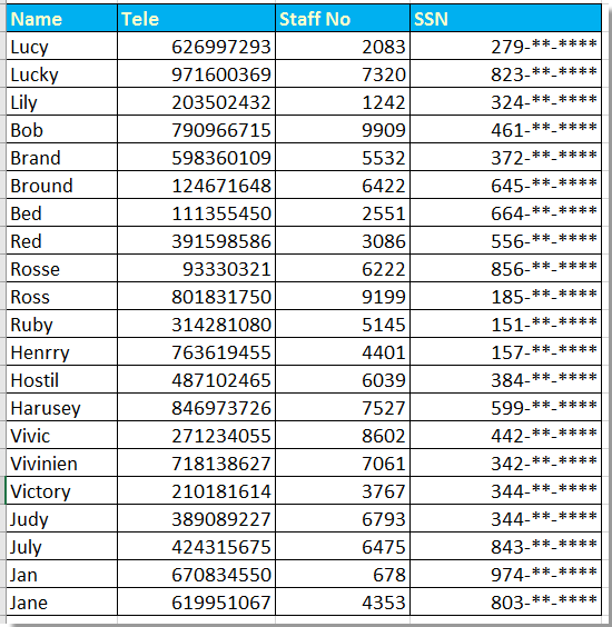
3. klik OK, nu er delnumre, du valgte, blevet skjult.

Bemærk: Den afrunder tallet, hvis det fjerde nummer er større end eller eaqul til 5.


pil blå højre boble Delvist skjul tekst eller tal med formler

Med ovenstående metode kan du kun skjule delnumre, hvis du vil skjule delnumre eller tekster, kan du gøre som nedenfor:

Her skjuler vi de første 4 numre af pasnummeret.

Vælg en tom celle ved siden af ​​pasnummeret, F22 for eksempel, indtast denne formel = "****" & HØJRE (E22,5), og træk derefter håndtaget til autofyldning over den celle, du har brug for for at anvende denne formel.
doc skjul delvist 4

Tip:

Hvis du vil skjule de sidste fire tal, skal du bruge denne formel, = VENSTRE (H2,5) & "****"

Hvis du vil skjule de tre midterste tal, skal du bruge dette = VENSTRE (H2,3) & "***" & HØJRE (H2,3)

Bedste kontorproduktivitetsværktøjer

🤖 Kutools AI Aide: Revolutionér dataanalyse baseret på: Intelligent udførelse   |  Generer kode  |  Opret brugerdefinerede formler  |  Analyser data og generer diagrammer  |  Aktiver Kutools funktioner...
Populære funktioner: Find, fremhæv eller identificer dubletter   |  Slet tomme rækker   |  Kombiner kolonner eller celler uden at miste data   |   Runde uden formel ...
Super opslag: VLookup med flere kriterier    Multiple Value VLookup  |   VOpslag på tværs af flere ark   |   Fuzzy Lookup ....
Avanceret rulleliste: Opret hurtigt rulleliste   |  Afhængig rulleliste   |  Multivælg rulleliste ....
Column Manager: Tilføj et bestemt antal kolonner  |  Flyt kolonner  |  Skift synlighedsstatus for skjulte kolonner  |  Sammenlign områder og kolonner ...
Fremhævede funktioner: Grid fokus   |  Designvisning   |   Stor Formel Bar    Arbejdsbog & Ark Manager   |  Ressourcebibliotek (Autotekst)   |  Datovælger   |  Kombiner regneark   |  Krypter/Dekrypter celler    Send e-mails efter liste   |  Superfilter   |   Specielt filter (filter fed/kursiv/gennemstreget...) ...
Top 15 værktøjssæt12 tekst Værktøjer (tilføje tekst, Fjern tegn, ...)   |   50 + Chart Typer (Gantt kort, ...)   |   40+ Praktisk formler (Beregn alder baseret på fødselsdag, ...)   |   19 Indsættelse Værktøjer (Indsæt QR-kode, Indsæt billede fra sti, ...)   |   12 Konvertering Værktøjer (Tal til ord, Valutaomregning, ...)   |   7 Flet og del Værktøjer (Avancerede kombinere rækker, Opdel celler, ...)   |   ... og mere

Overlad dine Excel-færdigheder med Kutools til Excel, og oplev effektivitet som aldrig før. Kutools til Excel tilbyder over 300 avancerede funktioner for at øge produktiviteten og spare tid.  Klik her for at få den funktion, du har mest brug for...

Beskrivelse


Fanen Office bringer en grænseflade til et kontor med Office, og gør dit arbejde meget lettere

  • Aktiver redigering og læsning af faner i Word, Excel, PowerPoint, Publisher, Access, Visio og Project.
  • Åbn og opret flere dokumenter i nye faner i det samme vindue snarere end i nye vinduer.
  • Øger din produktivitet med 50 % og reducerer hundredvis af museklik for dig hver dag!
Comments (21)
No ratings yet. Be the first to rate!
This comment was minimized by the moderator on the site
I have 1. Name, so I want to remove "1." Please suggest.
This comment was minimized by the moderator on the site
Is there any command for format cell, to hide the intended value in cell, that containt with charecters. eg. G1234567Q and after applied the format it would be G****567Q ?Note: I am asking to know the cell format not the formula? Thanks in advance!
This comment was minimized by the moderator on the site
If I have a listing of Name with different length, and want to set as "B*** P***" for "Brad Pitt", "M******* Y*** C*** K****" for "Michelle Yeoh Choo Kheng", how can I do it with formula?
p     JL
This comment was minimized by the moderator on the site
have you found a solution? i would also like to know the answer to this. thank you
This comment was minimized by the moderator on the site
Can replace all but the first char with this: =REPLACE(CELL,2,LEN(CELL),REPT("*",LEN(CELL)))
This comment was minimized by the moderator on the site
If I have a number and alphabet set like S1234567A and want to put as S****567A, what formula is usable?
This comment was minimized by the moderator on the site
=REPLACE(CELL,2,4,"****")
This comment was minimized by the moderator on the site
=REPLACE(CELL,1,LEN(CELL)-4,REPT("X",LEN(CELL)-4))is the better version as here you can mask text with variable length
This comment was minimized by the moderator on the site
Hi I tried this but does not seem to work.
This comment was minimized by the moderator on the site
Great solution!
This comment was minimized by the moderator on the site
How can we use format cell to remove the first few characters? For ex: 12,345.67 = **,345.67
This comment was minimized by the moderator on the site
how can i unhide the numbers again
This comment was minimized by the moderator on the site
Hi, sunil, if you use the Format Cells function to hide part of string, when you want to unhide them again, just format the cells as general.
This comment was minimized by the moderator on the site
Nice Sir, Its working
This comment was minimized by the moderator on the site
Sorry, I meant D22
This comment was minimized by the moderator on the site
I am not sure how you wrote the formula Dean, but =LEFT(F22,3)&"-**-****" shows 278-**-**** for me... Maybe check other formats on your destination cell?
This comment was minimized by the moderator on the site
Sorry I did not get your question, could you give me a screenshot or other more information to decribe it?
This comment was minimized by the moderator on the site
Your SSN example fails, in that it rounds up the number, rather than hiding the non-visible placings. In you example, 278-53-6128 is displayed as 279-**-****!
This comment was minimized by the moderator on the site
Sorry, could you give me more information about the fails in your examples? Because it works always in my examples.
This comment was minimized by the moderator on the site
Dean is correct, the image you are using for the example shows staff no 2083 having the social security number of 278536128 but the hidden version starts with 279. The formula itself works, just the first row in the example image is incorrect.
This comment was minimized by the moderator on the site
Thanks for the reminder. The format cell method will round up the number if the fourth number is larger than 5.
There are no comments posted here yet
Please leave your comments in English
Posting as Guest
×
Rate this post:
0   Characters
Suggested Locations