Gå til hovedindhold

Hvordan vises det første element på rullelisten i stedet for tomt?

doc drop down list standard til top 1

Rullelisten i et regneark kan hjælpe os med at gøre det lettere at indtaste data, vi skal bare vælge emnerne uden at skrive dem en efter en. Men engang, når du klikker på rullelisten, springer den først til de tomme emner i stedet for det første dataelement som vist på følgende skærmbillede, dette kan skyldes at slette kildedataene i slutningen af ​​listen. Det kan være irriterende, at du skal rulle tilbage til toppen af ​​en lang liste for hver tomme datavalideringscelle. Denne artikel vil jeg tale om, hvordan man altid viser det første element i rullelisten.

Vis det første element i rullelisten i stedet for tomt med datavalideringsfunktionen

Vis automatisk det første element i rullelisten i stedet for tomt med VBA-kode


pil blå højre boble Vis det første element i rullelisten i stedet for tomt med datavalideringsfunktionen

For at opnå dette job skal du faktisk anvende en bestemt formel, når du opretter en rulleliste, skal du gøre som følger:

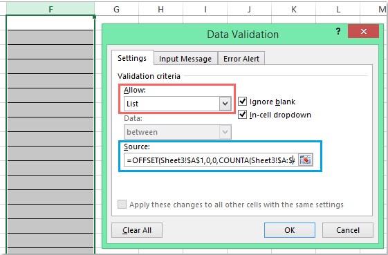
1. Vælg de celler, hvor du vil indsætte rullelisten, og klik på data > Datavalidering > Datavalidering, se skærmbillede:

doc drop down list standard til top 2

2. I poppet ud Datavalidering under dialogboksen Indstillinger fanebladet, vælg Liste fra Tillad sektion, og indtast derefter denne formel: = OFFSET (Ark3! $ A $ 1,0,0, COUNTA (Ark3! $ A: $ A) -1,1) ind i Kilde tekstboks, se skærmbillede:

Bemærk: I denne formel Sheet3 er regnearket indeholder kildedatalisten, og A1 er den første celleværdi på listen.

doc drop down list standard til top 3

3. Klik derefter på OK knap, nu, når du klikker på rullelistecellerne, vises det første dataelement altid øverst, om der er celleværdier slettet i slutningen af ​​kildedataene, se skærmbillede:

doc drop down list standard til top 4


pil blå højre boble Vis automatisk det første element i rullelisten i stedet for tomt med VBA-kode

Her kan jeg også introducere en VBA-kode, som kan hjælpe dig med at vise det første element i rullelisten automatisk, når du klikker på datavalideringscellerne.

1. Efter indsættelse af rullelisten skal du vælge regnearkfanen, der indeholder rullelisten, og højreklik for at vælge Vis kode fra genvejsmenuen for at gå til Microsoft Visual Basic til applikationer vindue, og kopier og indsæt derefter følgende kode i modulet:

VBA-kode: Vis automatisk det første dataelement i rullelisten:

Private Sub Worksheet_SelectionChange(ByVal Target As Range)
'Updateby Extendoffice 20160725
    Dim xFormula As String
    On Error GoTo Out:
    xFormula = Target.Cells(1).Validation.Formula1
    If Left(xFormula, 1) = "=" Then
        Target.Cells(1) = Range(Mid(xFormula, 1)).Cells(1).Value
    End If
Out:
End Sub

doc drop down list standard til top 5

2. Gem og luk derefter kodevinduet, og når du klikker på rullelistecellen, vises det første dataelement med det samme.

Bedste kontorproduktivitetsværktøjer

🤖 Kutools AI Aide: Revolutionér dataanalyse baseret på: Intelligent udførelse   |  Generer kode  |  Opret brugerdefinerede formler  |  Analyser data og generer diagrammer  |  Aktiver Kutools funktioner...
Populære funktioner: Find, fremhæv eller identificer dubletter   |  Slet tomme rækker   |  Kombiner kolonner eller celler uden at miste data   |   Runde uden formel ...
Super opslag: VLookup med flere kriterier    Multiple Value VLookup  |   VOpslag på tværs af flere ark   |   Fuzzy Lookup ....
Avanceret rulleliste: Opret hurtigt rulleliste   |  Afhængig rulleliste   |  Multivælg rulleliste ....
Column Manager: Tilføj et bestemt antal kolonner  |  Flyt kolonner  |  Skift synlighedsstatus for skjulte kolonner  |  Sammenlign områder og kolonner ...
Fremhævede funktioner: Grid fokus   |  Designvisning   |   Stor Formel Bar    Arbejdsbog & Ark Manager   |  Ressourcebibliotek (Autotekst)   |  Datovælger   |  Kombiner regneark   |  Krypter/Dekrypter celler    Send e-mails efter liste   |  Superfilter   |   Specielt filter (filter fed/kursiv/gennemstreget...) ...
Top 15 værktøjssæt12 tekst Værktøjer (tilføje tekst, Fjern tegn, ...)   |   50 + Chart Typer (Gantt kort, ...)   |   40+ Praktisk formler (Beregn alder baseret på fødselsdag, ...)   |   19 Indsættelse Værktøjer (Indsæt QR-kode, Indsæt billede fra sti, ...)   |   12 Konvertering Værktøjer (Tal til ord, Valutaomregning, ...)   |   7 Flet og del Værktøjer (Avancerede kombinere rækker, Opdel celler, ...)   |   ... og mere

Overlad dine Excel-færdigheder med Kutools til Excel, og oplev effektivitet som aldrig før. Kutools til Excel tilbyder over 300 avancerede funktioner for at øge produktiviteten og spare tid.  Klik her for at få den funktion, du har mest brug for...

Beskrivelse


Fanen Office bringer en grænseflade til et kontor med Office, og gør dit arbejde meget lettere

  • Aktiver redigering og læsning af faner i Word, Excel, PowerPoint, Publisher, Access, Visio og Project.
  • Åbn og opret flere dokumenter i nye faner i det samme vindue snarere end i nye vinduer.
  • Øger din produktivitet med 50 % og reducerer hundredvis af museklik for dig hver dag!
Comments (10)
No ratings yet. Be the first to rate!
This comment was minimized by the moderator on the site
=OFFSET(Sheet3!$A$1,0,0,COUNTA(Sheet3!$A:$A)+2-1,1) I added +2 to the equation and that worked for me.
This comment was minimized by the moderator on the site
For the VDA code, how can I have only a certain cell range show the first item in the drop down list? Thank you in advance.
This comment was minimized by the moderator on the site
Hi, Akrupa,To solve your problem, maybe the following VBA code can help you:

<div data-tag="code">Private Sub Worksheet_SelectionChange(ByVal Target As Range)
'Updateby Extendoffice 20211206
Dim xFormula As String
Dim xRg As Range
Dim xStr As String
Dim xIndex As Integer
xIndex = 2 'Here indicates the cell number of the original data,for example,the original data is A1:A10, to display the A2 cell value, please write 2 here.
On Error GoTo Out:
xFormula = Target.Cells(1).Validation.Formula1
If Left(xFormula, 1) = "=" Then
If Target.Value <> "" Then Exit Sub
xStr = Mid(xFormula, 2)
Set xRg = Application.Range(xStr)
Target.Cells(1) = xRg.Cells(xIndex).Value
End If
Out:
End Sub
Please try, hope it can help you!
This comment was minimized by the moderator on the site
Better but not quite. Using the =OFFSET(Sheet3!$A$1,0,0,COUNTA(Sheet3!$A:$A)-1,1) method eliminates the blanks but still starts you at the bottom of the very long list. I want it to start at the top of the list.
This comment was minimized by the moderator on the site
Once again, you save the day! Thanks!
This comment was minimized by the moderator on the site
Doesn't work for me. I keep getting an error message that says, "There's a problem with this formula. Not trying to type a formula? When the first character is an equal (+) or minus (-) sign, Exel thinks it's a formula.... To get around this, type an apostrophe (') first..."
This comment was minimized by the moderator on the site
Hello!

How can I set a data validation list such that if the drop down value in the cell is deleted, the cell will automatically show a default value (i.e. "-Select-")?

For example, I have a worksheet with multiple drop down lists that I want to show a default value of "-Select-" once the sheet is opened. A user will select values from the lists that will impact the result of calculations throughout the entire spreadsheet. A user may accidentally "delete" the cell contents of the lists. If this happens, rather than the cell becoming blank, I want the cell to show a default value of "-Select-". This scenario occurs in multiple random locations throughout the spreadsheet, not just in one localized place.

I was able to find the following VBA code so far, but it only applies the concept over a range, rather than just individual cells that contain drop down lists. The problem with what I have coded so far is that every single blank cell in the range ends up with "-Select-" in it. Some of the lists are in ranges, but some are also scattered throughout the sheet. The problem I'm having with my current code is that every single blank cell in the range ends up with "-Select-" in it. I'm trying to get this to apply over the entire worksheet to ONLY cells that are drop down lists.

Is what I'm trying to accomplish even possible?

Example file can be found here:
https://drive.google.com/file/d/1VoO8VgFs3IJ0ALwqfk0i8gt69UE4vEKW/view?usp=sharing

Example code:

Option Explicit

Private Sub Worksheet_Change(ByVal Target As Range)
Dim cel As Range
' If Target.Cells.Count > 1 Then Exit Sub 'turning this off allows multiple cells to be selected and deleted at the same time
If Not Intersect(Target, Range("f2:p17")) Is Nothing Then
For Each cel In Range("f2:p17")
Application.EnableEvents = False
If IsEmpty(cel.Value) Then cel.Value = "-Select-"
Next cel
End If
Application.EnableEvents = True
End Sub


Thanks in advance!
This comment was minimized by the moderator on the site
How can I set a data validation list such that if the drop down value in the cell is deleted, the cell will automatically show the a default value (i.e. "-Select-")?

For example, I have a worksheet with multiple drop down lists that I want to show a default value of "-Select-" once the sheet is opened. A user will select values from the lists that will impact the result of calculations throughout the entire spreadsheet. A user may accidentally "delete" the cell contents. If this happens, rather than the cell becoming blank, I want the cell to show a default value of "-Select-". This scenario occurs in multiple random locations throughout the spreadsheet, not just in one localized place.

I was able to come up with the following VBA code so far, but I've only figured out how to apply the concept over a range, rather than just cells that contain a drop down list. The problem with what I have coded so far is that every single blank cell in the range ends up with "-Select-" in it.

Option Explicit

Private Sub Worksheet_Change(ByVal Target As Range)
Dim cel As Range
' If Target.Cells.Count > 1 Then Exit Sub
If Not Intersect(Target, Range("f2:p17")) Is Nothing Then
For Each cel In Range("f2:p17")
Application.EnableEvents = False
If IsEmpty(cel.Value) Then cel.Value = "-Select-"
Next cel
End If
Application.EnableEvents = True
End Sub
This comment was minimized by the moderator on the site
select the cell in which you have put the listitem
the range for the listitem is "Opleiding"
in your VBA code:

selection.Value = Range("opleiding").Cells(2, 1)

the result is that the selected item of the listItem is the second item in the range "Opleiding"
This comment was minimized by the moderator on the site
After scroll down select to cells numeric data not come in series only first cell data come select 1,2 different cells and scroll down value not coming 1,2,3,4,5....... only first cell value coming 1,1,1,1,....
There are no comments posted here yet
Please leave your comments in English
Posting as Guest
×
Rate this post:
0   Characters
Suggested Locations