Du kan ændre de negative tal til positive tal med følgende trin:

1. Indtast nummer -1 i en tom celle, vælg derefter denne celle, og tryk på Ctrl + C nøgler til at kopiere den.

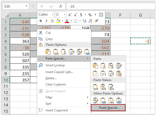
2. Vælg alle negative tal i området, højreklik, og vælg Indsæt særlige ... fra genvejsmenuen. Se skærmbillede:

Bemærkninger:
(1) Bedrift Ctrl nøgle, du kan vælge alle negative tal ved at klikke på dem en efter en;
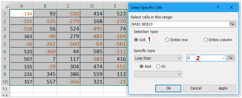
(2) Hvis du har Kutools til Excel installeret, kan du anvende dens Vælg Specielle celler funktion til hurtigt at vælge alle negative tal. Få en gratis prøveperiode!

3. Og a Indsæt specielt dialogboks vises, vælg Alle mulighed fra pasta, Vælg Gang mulighed fra Produktionklik OK. Se skærmbillede:

4. Alle valgte negative tal konverteres til positive tal. Slet nummeret -1, som du har brug for. Se skærmbillede:

Skift let negative tal til positive i det angivne interval i Excel

Sammenlignet med at fjerne det negative tegn fra celler en efter en manuelt, Kutools for Excel Skift værditegn funktion giver en ekstremt nem måde til hurtigt at ændre alle negative tal til positive i markeringen.

Som Excel-professionel kan du også køre VBA-koden for at ændre de negative tal til positive tal.

1. Tryk på Alt + F11-tasterne for at åbne vinduet Microsoft Visual Basic for Applications.

2. Der vises et nyt vindue. Klik på indsatte > Moduler, indtast derefter følgende koder i modulet:

Sub Positive
Dim Cel As Range
For Each Cel In Selection
If IsNumeric(Cel.Value) Then
Cel.Value = Abs(Cel.Value)
End If
Next Cel
End Sub

3. Klik derefter på Kør knappen eller tryk på F5 nøgle til at køre applikationen, og alle negative tal vil blive ændret til positive tal. Se skærmbillede:

De fleste af Excel-brugere ønsker ikke at bruge VBA-kode. Er der hurtige tricks til at ændre de negative tal til positive? Kutools til excel kan hjælpe dig let og komfortabelt med at opnå dette.

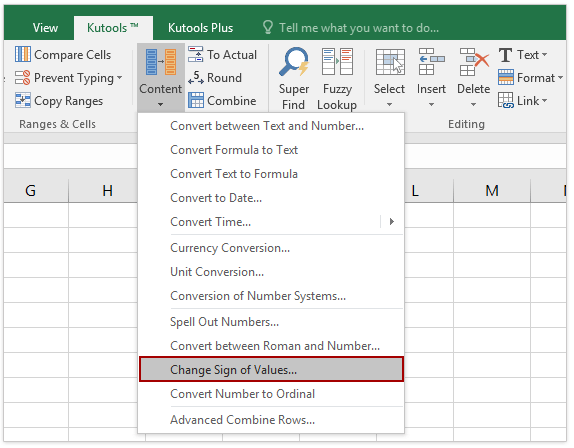
1. Vælg et interval inklusive de negative tal, du vil ændre, og klik på Kutools > Indhold > Skift værditegn.

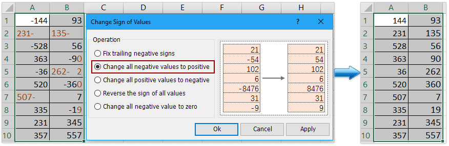
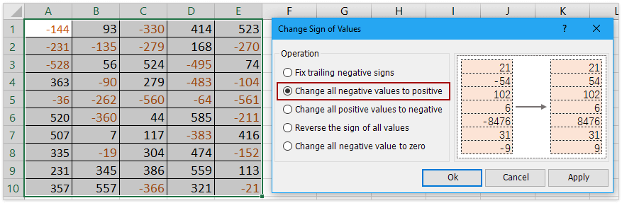
2. Check Skift alle negative værdier til positive under Produktion, og klik Ok. Se skærmbillede:

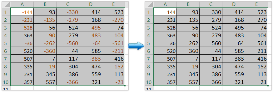
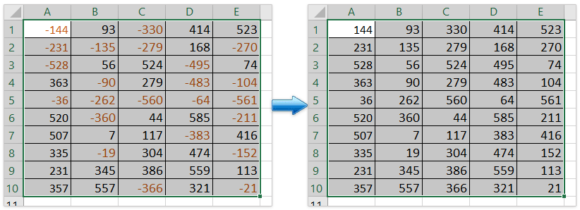
Nu vil du se alle negative tal skifte til positive tal som vist nedenfor:

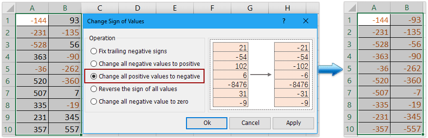
Bemærk: Med dette Skift tegn på værdier funktion, kan du også rette efterfølgende negative tegn, ændre alle positive tal til negative, vende tegnet på alle værdier og ændre alle negative værdier til nul. Få en gratis prøveperiode!

(1) Skift hurtigt alle positive værdier til negative i det angivne interval:

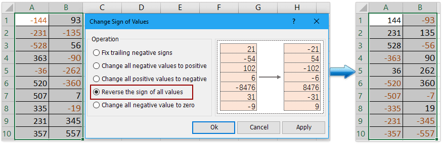
(2) Vend let tegnet på alle værdier i det angivne interval:

(3) Skift let alle negative værdier til nul i det angivne interval:

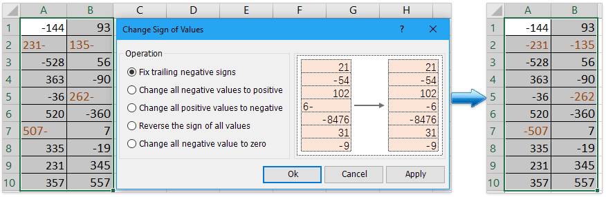
(4) Fastsæt let efterfølgende negative tegn i det specificerede interval:

Skift positive tal til negative

Omvendte tegn på værdier i celler

Fix efterfølgende negative tegn i celler

Skift negativt tal til nul