Hvordan sammenkædes celler, hvis samme værdi findes i en anden kolonne i Excel?
Som vist på skærmbilledet nedenfor, hvis du vil sammenkæde celler i den anden kolonne baseret på de samme værdier i den første kolonne, er der flere metoder, du kan bruge. I denne artikel vil vi introducere tre måder at udføre denne opgave på.

Sammenkæd celler, hvis samme værdi er med formler og filter
Følgende formler hjælper med at sammenkæde indholdet af de tilsvarende celler i en kolonne baseret på den samme værdi i en anden kolonne.
1. Vælg en tom celle udover den anden kolonne (her vælger vi celle C2), indtast formel = HVIS (A2 <> A1, B2, C1 & "," & B2) ind i formellinjen, og tryk derefter på Indtast nøgle.

2. Vælg derefter celle C2, og træk udfyldningshåndtaget ned til celler, du skal sammenkæde.

3. Indtast formlen = HVIS (A2 <> A3, CONCATENATE (A2, "," "", C2, "" ""), "") ind i celle D2, og træk Fill Handle ned til resten af cellerne.

4. Vælg celle D1, og klik data > filtre. Se skærmbillede:

5. Klik på drop-down pilen i celle D1, fjern markeringen af (Blank) og klik derefter på OK .

Du kan se, at cellerne sammenkædes, hvis de første kolonneværdier er de samme.

Bemærk: For at bruge ovenstående formler med succes skal de samme værdier i kolonne A være kontinuerlige.
Sammenkæd let celler, hvis den samme værdi er med Kutools til Excel (flere klik)
Metoden beskrevet ovenfor kræver oprettelse af to hjælpekolonner og involverer flere trin, hvilket kan være ubelejligt. Hvis du leder efter en enklere måde, kan du overveje at bruge Avancerede kombinere rækker værktøjet fra Kutools til Excel. Med blot et par klik giver dette værktøj dig mulighed for at sammenkæde celler ved hjælp af en specifik afgrænser, hvilket gør processen hurtig og problemfri.
Tip: Inden du anvender dette værktøj, bedes du installere Kutools til Excel for det første. Gå til gratis download nu.
- Vælg det område, du vil sammenkæde;
- Indstil kolonnen med de samme værdier som Primærnøgle kolonne.
- Angiv en separator for at kombinere cellerne.
- Klik OK.
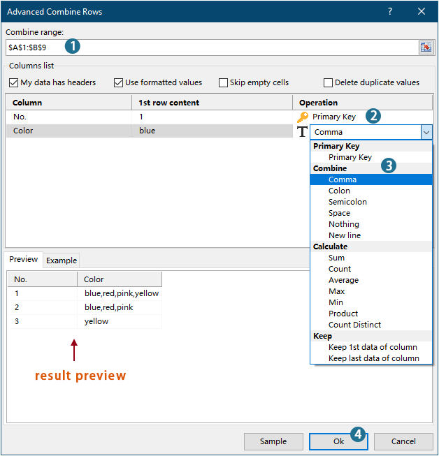
Resultat

- For at anvende denne funktion, venligst download og installer Kutools til Excel først.
- For at vide mere om denne funktion, tag et kig på denne artikel: Kombiner hurtigt de samme værdier eller dublerede rækker i Excel
Sammenkæd celler, hvis samme værdi er med VBA-kode
Du kan også bruge VBA-kode til at sammenkæde celler i en kolonne, hvis den samme værdi findes i en anden kolonne.
1. Trykke andre + F11 nøgler til at åbne Microsoft Visual Basic-applikationer vindue.
2. i Microsoft Visual Basic-applikationer vindue, skal du klikke på indsatte > Moduler. Kopier og indsæt derefter nedenstående kode i Moduler vindue.
VBA-kode: sammenkæd celler, hvis de samme værdier er
Sub ConcatenateCellsIfSameValues()
	Dim xCol As New Collection
	Dim xSrc As Variant
	Dim xRes() As Variant
	Dim I As Long
	Dim J As Long
	Dim xRg As Range
	xSrc    = Range("A1", Cells(Rows.Count, "A").End(xlUp)).Resize(, 2)
	Set xRg = Range("D1")
	On Error Resume Next
	For I = 2 To UBound(xSrc)
		xCol.Add xSrc(I, 1), TypeName(xSrc(I, 1)) & CStr(xSrc(I, 1))
	Next I
	On Error GoTo 0
	ReDim xRes(1 To xCol.Count + 1, 1 To 2)
	xRes(1, 1) = "No"
	xRes(1, 2) = "Combined Color"
	For I = 1 To xCol.Count
		xRes(I + 1, 1) = xCol(I)
		For J = 2 To UBound(xSrc)
			If xSrc(J, 1) = xRes(I + 1, 1) Then
				xRes(I + 1, 2) = xRes(I + 1, 2) & ", " & xSrc(J, 2)
			End If
		Next J
		xRes(I + 1, 2) = Mid(xRes(I + 1, 2), 2)
	Next I
	Set xRg = xRg.Resize(UBound(xRes, 1), UBound(xRes, 2))
	xRg.NumberFormat = "@"
	xRg = xRes
	xRg.EntireColumn.AutoFit
End SubNoter:
3. Tryk på F5 nøgle for at køre koden, så får du de sammenkædede resultater inden for det angivne interval.

Sammenkæd let celler, hvis den samme værdi er med Kutools til Excel
Bedste kontorproduktivitetsværktøjer
Overlad dine Excel-færdigheder med Kutools til Excel, og oplev effektivitet som aldrig før. Kutools til Excel tilbyder over 300 avancerede funktioner for at øge produktiviteten og spare tid. Klik her for at få den funktion, du har mest brug for...
")
Fanen Office bringer en grænseflade til et kontor med Office, og gør dit arbejde meget lettere
- Aktiver redigering og læsning af faner i Word, Excel, PowerPoint, Publisher, Access, Visio og Project.
- Åbn og opret flere dokumenter i nye faner i det samme vindue snarere end i nye vinduer.
- Øger din produktivitet med 50 % og reducerer hundredvis af museklik for dig hver dag!
")